Getting Started with AgentsMCP

Introduction to AgentsMCP

The AgentsMCP package provides a comprehensive implementation of the Agentic Neural Network Economic Model (ANNEM), featuring heterogeneous AI agents with neural decision-making capabilities, Model Context Protocol (MCP) communication, and dynamic network formation.

Installation

# Install from GitHub
devtools::install_github("avishekb9/AgentsMCP")

library(AgentsMCP)
#> Registered S3 method overwritten by 'quantmod':
#>   method            from
#>   as.zoo.data.frame zoo
library(ggplot2)
library(dplyr)
#> 
#> Attaching package: 'dplyr'
#> The following objects are masked from 'package:stats':
#> 
#>     filter, lag
#> The following objects are masked from 'package:base':
#> 
#>     intersect, setdiff, setequal, union

Quick Start Example

Let’s start with a simple ANNEM analysis using a small number of agents:

# Set seed for reproducibility
set_annem_seed(42)

# Run a basic ANNEM analysis
results <- run_annem_analysis(
  symbols = c("AAPL", "MSFT"),
  n_agents = 100,
  n_steps = 50,
  save_results = FALSE,
  verbose = FALSE
)

# View summary
annem_summary(results)

Understanding Agent Types

ANNEM implements six different types of heterogeneous agents:

Neural Momentum: Trend-following agents with neural network enhancement
Contrarian AI: Mean-reversion agents with AI-based signals
Fundamentalist ML: Technical analysis agents with machine learning
Adaptive Noise: Random strategy agents with adaptive learning
Social Network: Peer influence and herding behavior agents
Meta Learning: MAML-inspired strategy adaptation agents

Creating Individual Agents

# Create different types of agents
momentum_agent <- create_annem_agent("agent_001", "neural_momentum", 1000000)
contrarian_agent <- create_annem_agent("agent_002", "contrarian_ai", 1000000)

# Display agent properties
cat("Momentum Agent:\n")
#> Momentum Agent:
cat("- ID:", momentum_agent$id, "\n")
#> - ID: agent_001
cat("- Type:", momentum_agent$type, "\n")
#> - Type: neural_momentum
cat("- Wealth:", scales::dollar(momentum_agent$wealth), "\n")
#> - Wealth: $1,000,000
cat("- Risk Tolerance:", round(momentum_agent$risk_tolerance, 3), "\n\n")
#> - Risk Tolerance: 0.165

cat("Contrarian Agent:\n")
#> Contrarian Agent:
cat("- ID:", contrarian_agent$id, "\n")
#> - ID: agent_002
cat("- Type:", contrarian_agent$type, "\n")
#> - Type: contrarian_ai
cat("- Wealth:", scales::dollar(contrarian_agent$wealth), "\n")
#> - Wealth: $1,000,000
cat("- Risk Tolerance:", round(contrarian_agent$risk_tolerance, 3), "\n")
#> - Risk Tolerance: 0.682

Working with Market Data

The package can automatically download market data or work with synthetic data:

# Generate synthetic market data for testing
synthetic_data <- generate_synthetic_data(
  n_days = 100,
  n_assets = 2,
  annual_return = 0.08,
  annual_volatility = 0.20
)
#> Generated 100 days of synthetic data for 2 assets

cat("Generated", nrow(synthetic_data$prices), "days of data for", 
    ncol(synthetic_data$prices), "assets\n")
#> Generated 100 days of data for 2 assets
cat("Assets:", paste(synthetic_data$symbols, collapse = ", "), "\n")
#> Assets: Asset_1, Asset_2

# Plot synthetic price evolution
if (requireNamespace("ggplot2", quietly = TRUE)) {
  price_df <- data.frame(
    day = 1:nrow(synthetic_data$prices),
    price = synthetic_data$prices[, 1]
  )
  
  ggplot(price_df, aes(x = day, y = price)) +
    geom_line(color = "steelblue", size = 1) +
    labs(
      title = "Synthetic Asset Price Evolution",
      x = "Trading Day",
      y = "Price ($)"
    ) +
    theme_minimal()
}
#> Warning: Using `size` aesthetic for lines was deprecated in ggplot2 3.4.0.
#> ℹ Please use `linewidth` instead.
#> This warning is displayed once every 8 hours.
#> Call `lifecycle::last_lifecycle_warnings()` to see where this warning was
#> generated.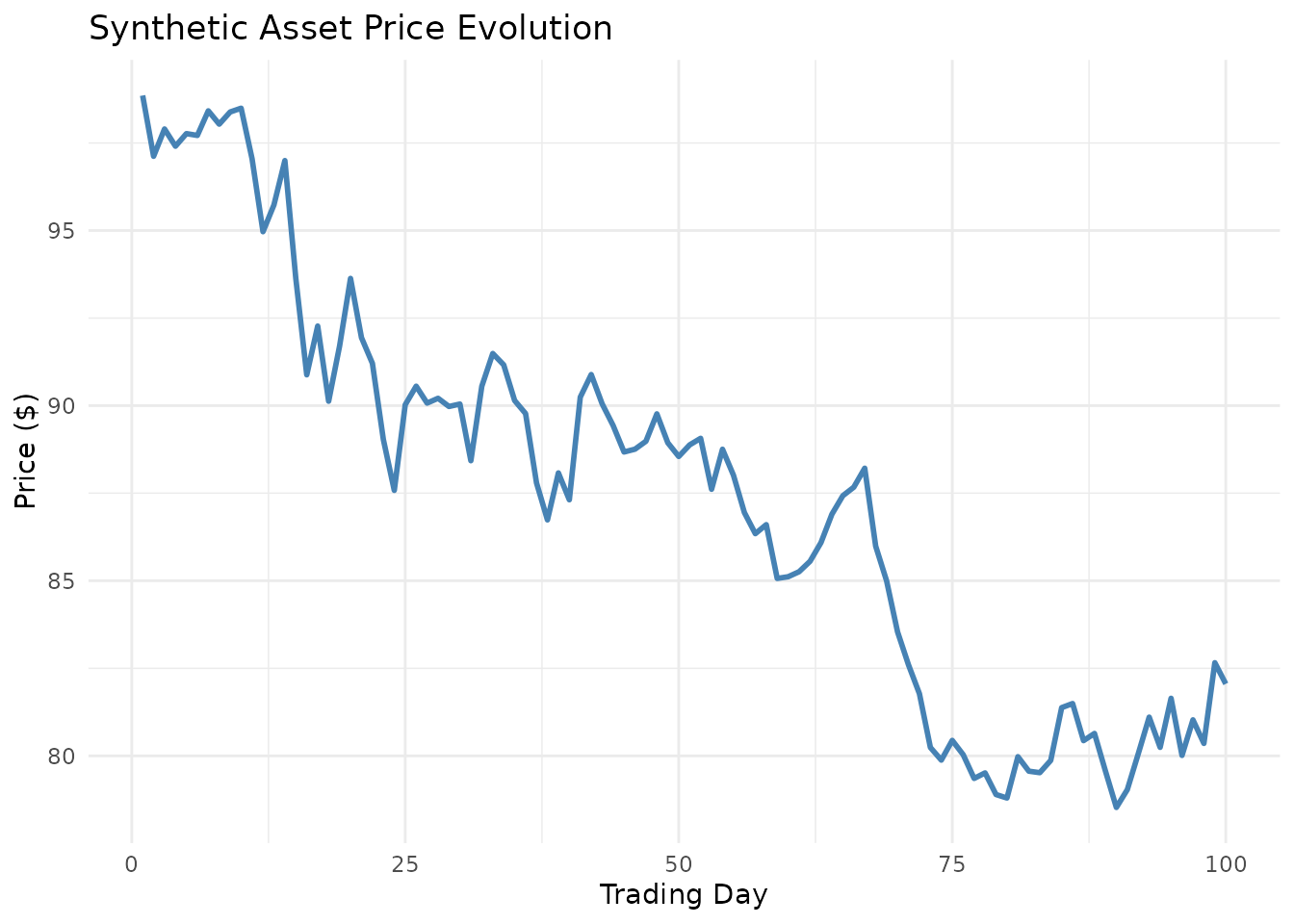

Creating and Running Market Simulations

Basic Market Creation

# Create a market environment
market <- create_annem_market(
  n_agents = 200,
  symbols = c("AAPL", "MSFT", "GOOGL")
)

# Examine the market
cat("Market created with", length(market$agents), "agents\n")
cat("Network density:", round(igraph::edge_density(market$network), 4), "\n")

# Check agent type distribution
agent_types <- sapply(market$agents, function(a) a$type)
type_distribution <- table(agent_types)
print(type_distribution)

Running Simulations

# Run simulation with the market
simulation_results <- market$run_simulation(n_steps = 100, verbose = TRUE)

# Analyze results
cat("Simulation completed with", simulation_results$n_steps, "steps\n")
cat("Agent decisions matrix dimensions:", 
    paste(dim(simulation_results$agent_decisions), collapse = " x "), "\n")
cat("Wealth evolution matrix dimensions:", 
    paste(dim(simulation_results$agent_wealth), collapse = " x "), "\n")

Performance Analysis

Agent Performance Metrics

# Analyze agent performance
agent_performance <- market$analyze_agent_performance()

# Summary by agent type
performance_summary <- agent_performance %>%
  group_by(agent_type) %>%
  summarise(
    count = n(),
    avg_return = mean(total_return) * 100,
    median_return = median(total_return) * 100,
    avg_sharpe = mean(sharpe_ratio),
    .groups = 'drop'
  ) %>%
  arrange(desc(avg_return))

print(performance_summary)

Network Analysis

# Analyze network evolution
network_metrics <- market$analyze_network_evolution()

# Display network evolution summary
cat("Network Evolution Summary:\n")
cat("- Initial density:", round(network_metrics$density[1], 4), "\n")
cat("- Final density:", round(tail(network_metrics$density, 1), 4), "\n")
cat("- Average clustering:", round(mean(network_metrics$clustering, na.rm = TRUE), 4), "\n")

Visualization

The package provides comprehensive visualization capabilities:

# Create performance plots
perf_plots <- plot_agent_performance(agent_performance)

# Display distribution plot
print(perf_plots$performance_dist)

# Create network evolution plots
network_plots <- plot_network_evolution(network_metrics)
print(network_plots$evolution)

# Create wealth dynamics plots
wealth_plots <- plot_wealth_dynamics(simulation_results)
print(wealth_plots$by_type)

Model Comparison and Validation

Benchmark Comparison

# Compare with traditional models
comparison_results <- market$compare_with_benchmarks()

print(comparison_results)

# Visualize comparison
comparison_plots <- plot_model_comparison(comparison_results)
print(comparison_plots$comparison)

Mathematical Framework Validation

# Validate implementation against mathematical framework
validation_results <- validate_annem_framework(market, simulation_results, agent_performance)

# Display validation summary
passed_tests <- sum(validation_results$Validation_Status == "PASS")
total_tests <- nrow(validation_results)

cat("Framework Validation Results:\n")
cat("Tests passed:", passed_tests, "out of", total_tests, "\n")

# Show any failed tests
failed_tests <- validation_results[validation_results$Validation_Status != "PASS", ]
if (nrow(failed_tests) > 0) {
  cat("\nTests requiring attention:\n")
  for (i in 1:nrow(failed_tests)) {
    cat("-", failed_tests$Metric[i], ":", failed_tests$Validation_Status[i], "\n")
  }
}

Advanced Configuration

Custom Agent Distributions

# Get default configuration
config <- get_annem_config()

cat("Default Agent Types:\n")
#> Default Agent Types:
for (i in 1:length(config$agent_types)) {
  cat("-", config$agent_types[i], ":", 
      scales::percent(config$agent_distribution[i]), "\n")
}
#> - neural_momentum : 20% 
#> - contrarian_ai : 15% 
#> - fundamentalist_ml : 18% 
#> - adaptive_noise : 12% 
#> - social_network : 25% 
#> - meta_learning : 10%

cat("\nDefault Parameters:\n")
#> 
#> Default Parameters:
cat("- Default agents:", config$default_n_agents, "\n")
#> - Default agents: 1000
cat("- Default steps:", config$default_n_steps, "\n")
#> - Default steps: 250
cat("- Risk-free rate:", scales::percent(config$risk_free_rate), "\n")
#> - Risk-free rate: 2%

Performance Optimization

For large-scale simulations, consider these optimization strategies:

# For testing and development
quick_results <- run_annem_analysis(
  symbols = c("AAPL"),
  n_agents = 50,
  n_steps = 25,
  save_results = FALSE
)

# For production analysis
production_results <- run_annem_analysis(
  symbols = c("AAPL", "MSFT", "GOOGL", "TSLA", "NVDA"),
  n_agents = 1000,
  n_steps = 250,
  save_results = TRUE,
  output_dir = "annem_production_results"
)

Error Handling and Troubleshooting

Common Issues and Solutions

Internet Connection: If market data download fails, use synthetic data:

# Fallback to synthetic data
tryCatch({
  real_data <- load_market_data(c("AAPL", "MSFT"))
}, error = function(e) {
  cat("Market data download failed, using synthetic data\n")
  real_data <- generate_synthetic_data(n_days = 252, n_assets = 2)
})

Memory Issues: Reduce simulation size for large analyses:

# Check available memory and adjust parameters accordingly
memory_limit <- as.numeric(gsub("[^0-9.]", "", memory.size(max = TRUE)))

if (memory_limit < 8000) {  # Less than 8GB
  n_agents <- 500
  n_steps <- 100
} else {
  n_agents <- 1000
  n_steps <- 250
}

cat("Using", n_agents, "agents and", n_steps, "steps based on available memory\n")

Next Steps

Explore the Advanced Modeling vignette for sophisticated analyses
Check out the Network Analysis vignette for detailed network studies
Review the Visualization Guide for comprehensive plotting options
Visit the package documentation for complete function references

References

Farmer, J. D., & Foley, D. (2009). The economy needs agent-based modelling. Nature, 460(7256), 685-686.
Jackson, M. O. (2008). Social and economic networks. Princeton University Press.
Billio, M., Getmansky, M., Lo, A. W., & Pelizzon, L. (2012). Econometric measures of connectedness and systemic risk in the finance and insurance sectors. Journal of Financial Economics, 104(3), 535-559.

Avishek Bhandari

2025-06-25